Building a Bayesian Network from Actuarial Data

Extracting causal structure from claims and underwriting data

Don’t mistake the forest for trees. Image generated with Leonardo AI

On Tuesday, we talked about the strategic value of causal thinking: moving from “what happened?” to “what should we do?” Today, we’re going to build that capability. We’ll construct a causal model of an insurance underwriting system using a Bayesian network, learn its parameters from data, and use it to answer the kinds of strategic questions that matter in the boardroom.

If you’re not familiar with Bayesian networks, don’t worry. They’re not as intimidating as they sound. At their core, they’re a way of encoding causal relationships between variables and then using those relationships to make probabilistic inferences. For actuaries, they’re particularly useful because they let you combine domain expertise (what you know about insurance) with data (what the numbers tell you), and they produce interpretable results—you can see the causal structure, not just a black box prediction.

Why Bayesian Networks for Insurance?

There are several reasons Bayesian networks are well-suited to actuarial work. First, they’re causal by design. Unlike correlation-based models, which tell you what’s associated with what, Bayesian networks encode explicit causal relationships. You define the structure (the DAG, or directed acyclic graph) that represents how you believe the insurance system works, and then the network learns the strength of those relationships from data.

Second, they’re interpretable. You can visualize the network, see the causal chains, and understand exactly how one variable influences another. This is crucial when you’re trying to communicate insights to non-technical stakeholders in the boardroom.

Third, they’re flexible. You can use them for inference in either direction. Given an underwriting profile, you can predict claims outcomes. But you can also work backwards: given observed claims, you can infer what might have caused them. And you can run scenario analysis: “What if we change this variable? How does that cascade through the system?”

Fourth, they handle missing data and uncertainty gracefully. Insurance data is often incomplete, and Bayesian networks are built to work with that. They also naturally express uncertainty in their outputs—not just point estimates, but probability distributions.

The Use Case: Motor Insurance Underwriting

Let’s make this concrete. We’re going to model a simplified motor insurance system with the following variables:

• Underwriting characteristics: Driver age, territory (urban/suburban/rural), coverage type (liability/comprehensive/full)

• Premium: The price charged for the policy

• Claims frequency: The probability that a claim will occur

• Claims severity: The size of the claim if it occurs

• Total claims: The aggregate claims amount

• Loss ratio: Total claims divided by premium

• Reserves: The amount set aside to cover future claims

These variables have causal relationships. Underwriting decisions (age, territory, coverage) influence the premium we charge and the claims frequency we expect. Claims frequency and severity combine to determine total claims. Total claims and premium determine the loss ratio. And loss ratio, along with premium, influences how much we reserve.

This is a simplified version of how insurance actually works, but it’s realistic enough to be useful—and simple enough to understand.

Defining the Causal Structure

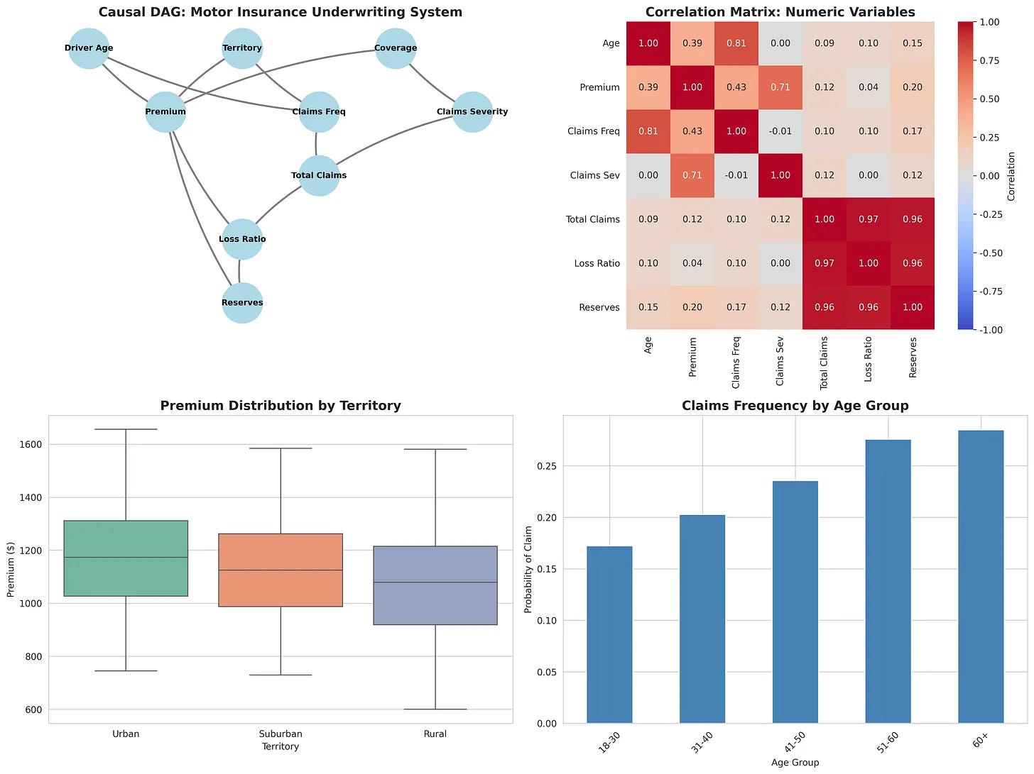
The first step is to define the DAG: the causal graph that represents these relationships. Here’s the conceptual structure:

Underwriting Characteristics (Age, Territory, Coverage)
    ↓
    ├→ Premium
    └→ Claims Frequency
        ↓
        ├→ Total Claims ←─ Claims Severity
        ↓
    Loss Ratio ←─ Premium
        ↓
    Reserves ←─ Premium

In code, this looks something like:

from pgmpy.models import BayesianNetwork
import pandas as pd

# Define the DAG structure
edges = [
    ('driver_age', 'premium'),
    ('driver_age', 'claims_frequency'),
    ('territory', 'premium'),
    ('territory', 'claims_frequency'),
    ('coverage_type', 'premium'),
    ('coverage_type', 'claims_severity'),
    ('claims_frequency', 'total_claims'),
    ('claims_severity', 'total_claims'),
    ('premium', 'loss_ratio'),
    ('total_claims', 'loss_ratio'),
    ('loss_ratio', 'reserves'),
    ('premium', 'reserves')
]

# Create the network
model = BayesianNetwork(edges)

This is where domain expertise comes in. You’re not letting the algorithm decide what causes what; you’re encoding your understanding of the insurance system. This is a critical step, because a wrong causal structure will lead to wrong inferences, no matter how good your data is.

Learning Parameters with bnlearn

Once you’ve defined the structure, the next step is to learn the parameters—the conditional probability tables (CPTs) that quantify the strength of each relationship. This is where bnlearn becomes invaluable.

What bnlearn does

bnlearn is a Python library specifically designed for Bayesian network learning and inference. Given your DAG and your data, it learns the CPTs automatically. But what makes it particularly useful for actuarial work is not just that it automates parameter learning, but how it does it and what options it gives you.

Here’s the conceptual workflow:

import bnlearn as bn

# Load your actuarial data
data = pd.read_csv('actuarial_data.csv')

# Fit the network to the data
model_fitted = bn.fit(model, data, estimator='BayesianEstimator')

What’s happening under the hood is that bnlearn is calculating, for each variable, the conditional probability distribution given its parents in the DAG. For example, it’s learning P(Premium | Driver Age, Territory, Coverage Type). It’s learning P(Claims Frequency | Driver Age, Territory). And so on. The result is a fully parameterized Bayesian network that encodes both your causal assumptions (the structure) and what the data tells you about the strength of those relationships (the parameters).

Why bnlearn is suited to insurance

There are several reasons bnlearn is particularly useful for actuarial applications:

First, it handles categorical and mixed data naturally. Insurance data is often categorical or mixed. You have categorical variables like territory, coverage type, and claim type. You have continuous variables like premium and claims amount. bnlearn works seamlessly with both. You can discretize continuous variables (bin them into categories) and the library handles the parameter learning without fuss. This is important because Bayesian networks traditionally work with discrete variables, and bnlearn makes that transition smooth.

Second, it offers multiple estimation methods. When learning parameters from data, you have choices about how to estimate the conditional probabilities. bnlearn supports several: maximum likelihood estimation (MLE), Bayesian estimation, and others. For actuarial work, Bayesian estimation is often preferable because it incorporates prior knowledge. If you have strong domain beliefs about certain relationships, you can encode them as priors, and the algorithm will weight the data accordingly. This is crucial in insurance, where you often have strong prior beliefs (e.g., “older drivers have higher claims frequency”) and you want the data to refine those beliefs, not overturn them.

Third, it integrates inference seamlessly. Once you’ve fitted the network, bnlearn provides inference engines that let you run probabilistic queries. The most common is variable elimination, which is efficient for networks of moderate size (which covers most actuarial applications). You can query the network in multiple directions: forward (given underwriting, predict claims), backward (given claims, infer underwriting), and counterfactual (what if we intervene on this variable?).

Fourth, it’s designed for interpretability. bnlearn outputs are transparent. You can inspect the learned CPTs, visualize the network, and understand exactly what the model learned. This is essential for regulatory and business contexts where you need to explain your models. Unlike deep learning approaches, there’s no black box. You can point to specific conditional probabilities and say “this is what the data told us about this relationship.”

Fifth, it handles missing data gracefully. Real actuarial data is often incomplete. bnlearn can work with missing values using expectation-maximization (EM) algorithms. Rather than discarding records with missing data or imputing them crudely, bnlearn learns the network structure and parameters while accounting for the missingness. This is particularly valuable in insurance, where missing data is common and often informative (e.g., a missing claims amount might indicate no claim occurred).

The estimation challenge in actuarial contexts

One subtle but important point: when you fit a Bayesian network to actuarial data, you’re making an assumption that the data-generating process is stationary—that the relationships you observe in historical data will hold in the future. This is often true for insurance, but not always. Market conditions change. Underwriting standards drift. Customer mix shifts. bnlearn doesn’t know about these shifts; it just learns from the data you give it.

This is why domain expertise is so critical. You need to validate the learned parameters against your domain knowledge. Does it make sense that urban drivers have 8% higher claims frequency? Does it make sense that comprehensive coverage increases severity by $500? If the learned relationships contradict your understanding, you need to investigate. Either your understanding is wrong (and the data is teaching you something), or your data is biased (and you need to be careful about how you use the model).

bnlearn makes this validation easier because the learned parameters are interpretable. You can see exactly what it learned and compare it to your expectations.

Making Strategic Inferences

Now you have a causal model. What can you do with it?

Inference Query 1: Prediction

Given an underwriting profile, what’s the expected claims outcome?

Here’s an idea of how that would look like in practice:

# Inference: Given a 45-year-old urban driver with comprehensive coverage,
# what's the probability of a claim?
evidence = {
    'driver_age': 45,
    'territory': 'Urban',
    'coverage_type': 'Comprehensive'
}

# Run inference
inferred_state = bn.inference.VariableElimination(model_fitted)
result = inferred_state.query(variables=['claims_frequency'], evidence=evidence)

This is useful for underwriting decisions. You’re not just using a black-box model; you’re using a causal model that you understand and can explain.

Inference Query 2: Causal Attribution

Why did we observe a particular outcome? Given that we observed high claims, what’s the most likely explanation?

# Inference: Given that we observed high loss ratio,
# what's the most likely driver profile?
evidence = {'loss_ratio': 'High'}

result = inferred_state.query(variables=['driver_age', 'territory'], evidence=evidence)

This is useful for root cause analysis. When something goes wrong (high loss ratio, reserve volatility), you can use the model to work backwards and identify the most likely causes.

Inference Query 3: Scenario Analysis

What if we change something? This is where causal inference really shines:

# Scenario: What if we tighten underwriting and only accept drivers under 50?
# How does that change our expected loss ratio?

# Baseline scenario
baseline = inferred_state.query(variables=['loss_ratio'])

# Intervention scenario
intervention = inferred_state.query(variables=['loss_ratio'], evidence={'driver_age': '<50'})

# Compare
print(f"Baseline loss ratio: {baseline}")
print(f"After intervention: {intervention}")

This is the strategic question: if we intervene on one variable, how does that cascade through the system? This is what you can’t answer with correlation-based models. You need causal reasoning.

The Data: Synthetic Actuarial Dataset

For this walkthrough, I’ve created a synthetic dataset with 5,000 records that reflects realistic actuarial relationships. The dataset includes driver age (normally distributed around 45), territory (urban/suburban/rural mix), coverage type (liability/comprehensive/full), and derived variables like premium, claims frequency, claims severity, total claims, loss ratio, and reserves.

The key feature of this synthetic data is that the causal relationships are explicit and realistic. Older drivers and urban territory increase both premium and claims frequency. Different coverage types have different severity profiles. Reserves scale with loss ratio and premium. This means when you fit a Bayesian network to this data, the learned relationships will match the true underlying causal structure—which is exactly what you want for learning and validation.

You can generate this dataset yourself with a simple script (the full code is available in the accompanying materials). The advantage of synthetic data is that you control the causal structure, so you can validate that bnlearn is learning the right relationships. Once you’re confident in the methodology, you can apply it to your own actuarial data.

What You Get

Once you’ve built and fitted your Bayesian network, you have a few key advantages:

Interpretability: You can visualize the network and see exactly how variables relate to each other. No black box. No feature importance scores that don’t make sense. Just causal relationships that you defined and that the data validated.

Explainability: When you make a decision based on the model, you can explain it. “We’re pricing this policy at $1,200 because the driver is 50 years old and lives in an urban area, which increases both premium and claims frequency according to our causal model.”

Scenario Analysis: You can run “what if” analyses that actually make sense. “If we tighten underwriting to exclude drivers over 60, our expected loss ratio would decrease by X%.” This is the language of strategy.

Adaptability: The framework works for any insurance domain. Motor, home, health, commercial—the structure changes, but the methodology is the same. You define the causal relationships, fit the network to your data, and run inferences.

A causal DAG (top left) and some exploratory data analysis (top right through bottom right) on our dummy dataset. Image by author

The Limitations

That said, Bayesian networks aren’t a silver bullet. A few things to keep in mind:

Structure matters more than data. If your DAG is wrong, no amount of data will fix it. This is why domain expertise is critical. You need to get the causal structure right, or your inferences will be misleading.

Discrete variables work best. Bayesian networks traditionally work with categorical variables. You can use continuous variables, but you often need to discretize them (bin them into categories), which loses information.

Scalability can be an issue. As you add more variables and more complex relationships, inference can become computationally expensive. For most actuarial applications this isn’t a problem, but it’s worth knowing.

You still need validation. Just because the model fits your data doesn’t mean it’s right. You need to validate the structure against domain expertise, test the inferences against holdout data, and be skeptical of surprising results.

Next Steps

If you want to build this yourself, here’s what you’d do:

1. Define your DAG: Sit down with domain experts and map out the causal relationships in your system. Draw it. Validate it.

2. Prepare your data: Get your actuarial data into a format that bnlearn can work with. Handle missing values, discretize continuous variables if needed.

3. Fit the network: Use bnlearn to learn the parameters from your data.

4. Validate: Test the inferences against your domain knowledge. Does it make sense? Are there surprising results that you need to investigate?

5. Deploy: Use the fitted network for underwriting decisions, scenario analysis, and strategic planning.

The libraries are free and well-documented. bnlearn is available on PyPI. pgmpy is another option if you want more control. Both work well for actuarial applications.

The Bigger Picture

What we’ve done here is bridge the gap between strategic insight and technical execution.

You have the data. You have the domain expertise. All you need is a framework for encoding that expertise and learning from the data. Bayesian networks, powered by bnlearn, provide exactly that framework.

The result isn’t just a better model. It’s a different way of thinking about your insurance system—not as a collection of correlations, but as a causal system where decisions have predictable consequences. And that’s the foundation of strategic decision-making.