

Active Learning Beats Brute Force Machine Learning
Teaching Machine Learning models to select the right training material is more efficient


When I was a student, my best learning never came from following the syllabus page by page. It came from curiosity. I enjoyed chasing the questions that interested me most, even if they jumped far ahead (or behind, or to the side) of the curriculum. I didn’t cover everything all the time, but I built a solid understanding of what really mattered, and I did it faster than many of my peers.
Machine learning can work the same way. Instead of force-feeding a model every possible example, what if we let it choose which data points it’s most uncertain about — the ones that really test its knowledge? That’s the idea behind Active Learning: a strategy where models guide their own education, zooming in on the boundaries that matter.
I was lucky enough to explore Active Learning during my PhD—I even coauthored a paper about it. These days, I’m coming back to it: It’s starting to help me quite a bit in sifting through data in finance, sustainability, and development—spaces in which additional data can be costly to get, so you need to do more (learn more!) with less.
The contrast of Active Learning is with brute-force learning: throwing every labeled point at a model and hoping for the best. It works, but it is wasteful. Labels are expensive, compute is costly, and much of the data adds little value. Active Learning reduces all of this waste: fewer labels and smarter selection means faster progress.
The Problem with Brute Force
The default approach in machine learning is feeding the model as much labeled data as possible, and hoping it figures things out. This brute-force strategy is reliable, but it’s also wasteful.
Most real datasets contain a lot of redundancy. Thousands of examples say essentially the same thing. Training on all of them doesn’t teach the model much more than training on a well-chosen subset.
What really matters are the edge cases, that is, the examples near the decision boundary where the model is most uncertain.
But brute force doesn’t do that. It just throws equal effort at trivial datapoints and at critical ones. It’s like asking a student to memorize every single line of a textbook, instead of encouraging them to focus on the concepts they find difficult or confusing. More effort, less insight.
In small, low-dimensional problems this inefficiency may not matter much. But as the number of features grows, brute force quickly becomes impractical. High-dimensional spaces explode in size, labels become expensive, and compute costs spiral upward.
Enter Active Learning
Active Learning takes the opposite approach. Instead of swallowing every data point blindly, the model learns to ask for the labels it finds most useful. In practice, this usually means focusing on the points where the model is least confident — right at the decision boundary, where it’s unsure which side a sample belongs to.
The intuition is simple: if the model is already 99% sure about an example, labeling it won’t change much. But if it’s 50/50, that label is gold. It teaches the model where its blind spots are, and those blind spots are often the exact contours that define the problem.
Mathematically, we can measure this uncertainty with a simple score. If the model predicts a probability y of belonging to a class, then the uncertainty is:
This expression peaks at 0.5 — the model’s “coin flip” zone — and drops to zero when the model is fully confident. By sampling the points with the highest uncertainty, Active Learning directs effort where it matters most.
The effect is the same as a curious student raising their hand when they don’t understand something: every answer they receive clears up a critical confusion. Over time, these questions add up to a deeper understanding, achieved with far fewer total lessons.
A Toy Example in Python
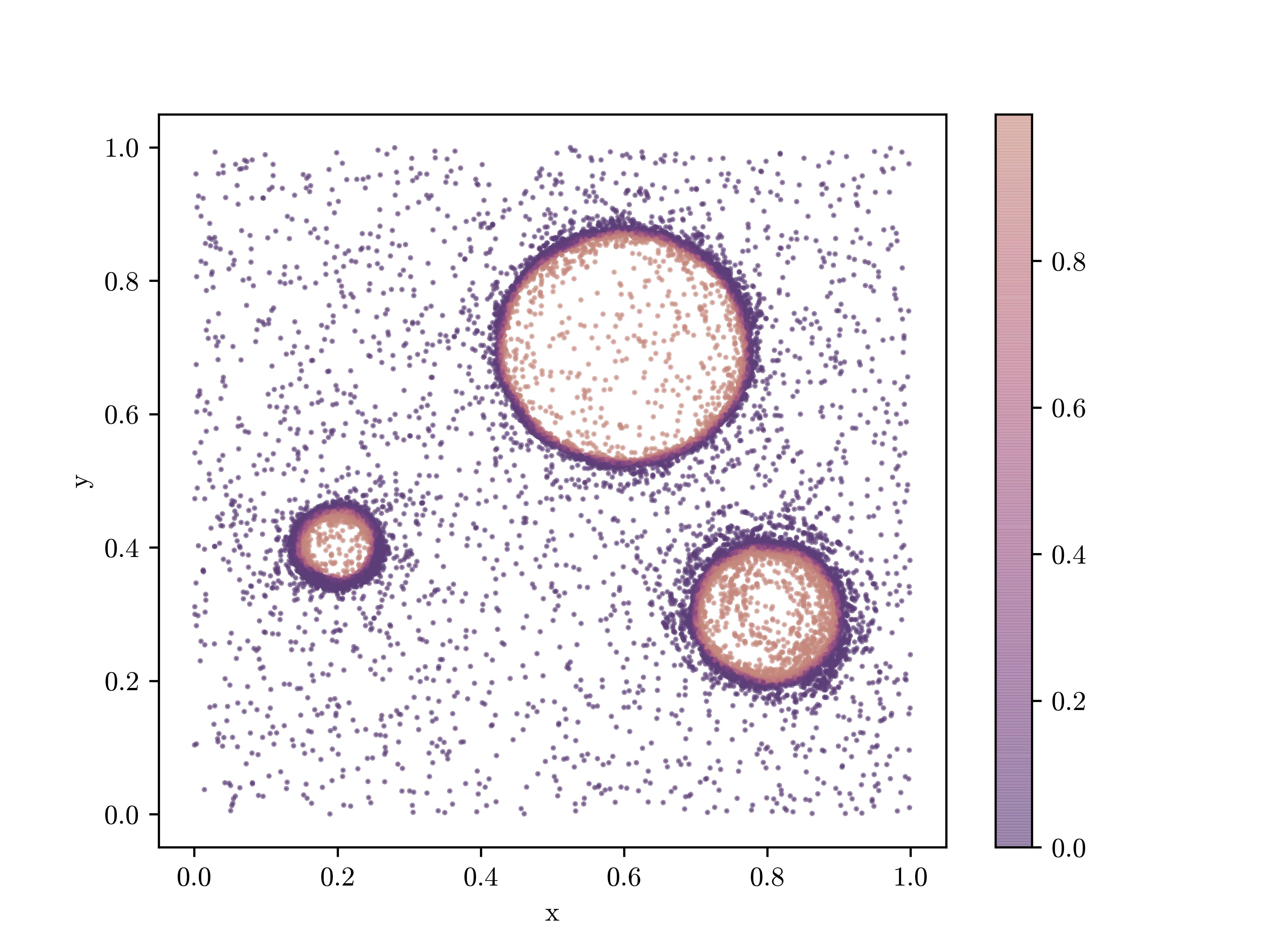
Let’s make this concrete with a simple toy dataset. We’ll use scikit-learn’s make_moons function, which generates two interleaving crescents of points. It’s a classic test case for binary classification because the two classes are not linearly separable — any model needs a curved decision boundary to get things right.
This setup is often used in tutorials because it’s just tricky enough to need a curved decision boundary, but still easy to visualize.
from sklearn.datasets import make_moons
X, y = make_moons(n_samples=10000, noise=0.35, random_state=42)
In plain English: this line gives us a synthetic dataset with 10,000 points. Each point belongs to one of two classes, but the separation isn’t perfectly clean — some points are noisy and blur the boundary.
To classify these points, we’ll use a support vector machine (SVM) with a curved (“RBF”) kernel. If you’re not familiar with SVMs, think of it as a flexible line-drawer: instead of a straight line, it can bend and wiggle to separate the two classes.
from sklearn.svm import SVC
clf = SVC(kernel="rbf", C=3.0, probability=True)
What matters here isn’t the details of the SVM, but that it can learn complex boundaries if given the right data.
Now comes the Active Learning part. The trick is to let the model tell us which points it finds hardest to classify. The technical way to measure this is with a probability: if the model is 99% sure a point belongs to class A, that label won’t change much. But if the model says it’s 50/50 between A and B, that label will be extremely valuable.
def uncertainty(x):
    p = clf.predict_proba(x)[:,1]
    return p*(1-p)   # highest when the model is least sure
In words: this little function scores each point by how “confused” the model is. Active Learning then picks the most confusing points first, asks for their labels, and retrains on those.
When we run this process side by side with random labeling (where points are chosen blindly), the difference becomes clear:
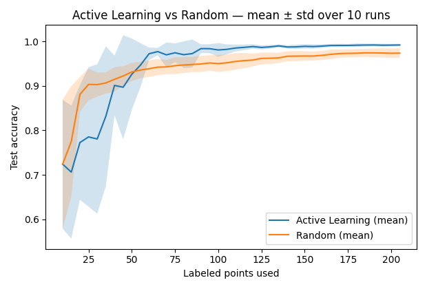
This is the payoff of letting the model follow its curiosity — focusing on what it doesn’t know, instead of repeating what it already does.
You can find the full code on GitHub.
Why It Works — and When It Doesn’t
The magic of Active Learning lies in where it spends its effort. Most datasets are full of “easy” points — ones that are obvious to classify. If a model already knows that 99 out of 100 positive examples look a certain way, labeling the hundredth doesn’t change much. Random sampling will happily keep feeding the model more of the same.
Active Learning takes a different route: it hunts for the hard cases. By focusing on points where the model is unsure, it sharpens the decision boundary much faster. In our toy moons example, these are the points that lie along the crescent edges, where the classes almost overlap. Labeling those points gives the model critical information, allowing it to generalize more efficiently.
That’s why in practice, you often see Active Learning reach a given accuracy with far fewer labeled examples than brute force. In domains where labeling is expensive — say, medical imaging, ESG disclosures, or fraud detection — this can save huge amounts of time and money.
But there are caveats. Active Learning isn’t a free lunch:
It needs a starting point. With zero labels, the model has no sense of what’s “uncertain.” You need at least a small seed set of labeled data to get the process going.
It can get stuck. If the model focuses too narrowly, it may miss rare or unusual cases that matter in the real world. That’s why many implementations add a “diversity” term, to make sure the selected points aren’t all clustered in the same place.
It’s sensitive to noise. If the data is messy or the labels themselves are inconsistent, Active Learning can sometimes chase false signals — asking for labels in areas that are confusing only because the underlying data is flawed.
It’s not always better in simple problems. On tiny or very easy datasets, random sampling may perform just as well (as we saw earlier when we first tested on a simple logistic regression). The real payoff comes in larger, high-dimensional spaces where brute force is infeasible.
In other words: Active Learning is at its best when labels are expensive, the decision boundary is complex, and you want to focus your resources on the places that matter most.
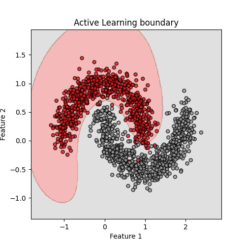
To make this even clearer, let’s look at what the model has actually learned. Below are two classifiers trained with the same number of labeled points: one chosen by Active Learning, the other chosen at random.
In the first picture above, Active Learning has focused its questions near the tricky crescent edges, and as a result the curved decision boundary closely follows the true separation between the two classes.
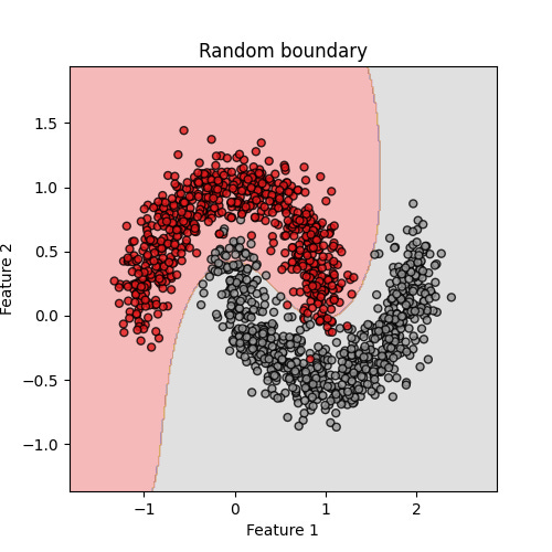
On the bottom picture, random sampling has wasted labels on easier points far from the boundary. The decision line cuts too sharply, misclassifying many points along the edge.
The contrast is striking: with the same labeling budget, Active Learning produces a boundary that is far more faithful to the underlying structure. In practice, this means better accuracy for fewer labels — a crucial advantage when data is costly to obtain.
Beyond 2D: The Real Payoff in High Dimensions
The two-dimensional moons are fun to look at, but they’re only a teaching tool. In real applications, data rarely lives in two dimensions. Finance, sustainability, medicine, physics — these are all high-dimensional worlds, where every observation comes with dozens, hundreds, or even thousands of features.
In low dimensions, brute force still works. You can plot the points, label a few hundred, and train a reasonable model. But in high dimensions, brute force breaks down. The space is simply too vast. The number of possible configurations grows exponentially, and the cost of labeling or simulating every case quickly becomes prohibitive.
This is exactly where Active Learning shines. By sampling only the most informative points, it avoids wasting effort on the huge regions the model already understands. Instead, it zeroes in on the boundaries that matter most — the edges where predictions flip from safe to risky, profitable to unprofitable, healthy to diseased.
I saw this firsthand in my own research. Traditional Monte Carlo scans wasted enormous effort on irrelevant regions of particle physics models. Active Learning, by contrast, honed in on the decision boundaries and found them with orders of magnitude fewer evaluations.
The same principle applies far beyond physics:
Finance: explore tipping points in stress-test models without brute-forcing every market scenario.
Sustainability: prioritize labeling the company disclosures that are genuinely ambiguous, instead of re-reading the obvious ones.
Medicine: focus radiologists’ attention on scans that algorithms find most uncertain, reducing workload while improving accuracy.
In short: while the toy moons dataset is a nice demo, the real payoff of Active Learning comes when the dimensions multiply and brute force is no longer an option.
The Bottom Line: Just Learn What You Want
Toy examples in two dimensions are fun to look at, but the real power of Active Learning shows up in high-dimensional problems — the kind we face in real datasets, from finance portfolios to sustainability disclosures to medical imaging. In those spaces, brute force quickly becomes impossible.
Active Learning offers a different path: let the model focus on the “hard questions,” where it’s uncertain, and ignore the easy or repetitive cases. This not only saves resources, it often uncovers the most interesting patterns — the boundaries where outcomes flip, where risk concentrates, or where scientific discovery lives.
For me, it echoes the way I’ve always learned best: by following what’s genuinely interesting, rather than absorbing everything indiscriminately. Models, like people, learn more by asking better questions than by following a pre-built curriculum.